Project Preparation: Threat Assessment for Protected Areas in Honduras
Andreas Petutschnig
2023-11-03
Last updated: 2023-11-03
Checks: 7 0
Knit directory: mapme.protectedareas/
This reproducible R Markdown analysis was created with workflowr (version 1.7.1). The Checks tab describes the reproducibility checks that were applied when the results were created. The Past versions tab lists the development history.
Great! Since the R Markdown file has been committed to the Git repository, you know the exact version of the code that produced these results.
Great job! The global environment was empty. Objects defined in the global environment can affect the analysis in your R Markdown file in unknown ways. For reproduciblity it’s best to always run the code in an empty environment.
The command set.seed(20210305) was run prior to running
the code in the R Markdown file. Setting a seed ensures that any results
that rely on randomness, e.g. subsampling or permutations, are
reproducible.
Great job! Recording the operating system, R version, and package versions is critical for reproducibility.
Nice! There were no cached chunks for this analysis, so you can be confident that you successfully produced the results during this run.
Great job! Using relative paths to the files within your workflowr project makes it easier to run your code on other machines.
Great! You are using Git for version control. Tracking code development and connecting the code version to the results is critical for reproducibility.
The results in this page were generated with repository version fa539f7. See the Past versions tab to see a history of the changes made to the R Markdown and HTML files.
Note that you need to be careful to ensure that all relevant files for
the analysis have been committed to Git prior to generating the results
(you can use wflow_publish or
wflow_git_commit). workflowr only checks the R Markdown
file, but you know if there are other scripts or data files that it
depends on. Below is the status of the Git repository when the results
were generated:
Ignored files:
    Ignored:    .RData
    Ignored:    .Rhistory
    Ignored:    .Rproj.user/
    Ignored:    analysis/threat_assessment_selva_maya_cache/
Note that any generated files, e.g. HTML, png, CSS, etc., are not included in this status report because it is ok for generated content to have uncommitted changes.
These are the previous versions of the repository in which changes were
made to the R Markdown
(analysis/threat_assessment_honduras.Rmd) and HTML
(docs/threat_assessment_honduras.html) files. If you’ve
configured a remote Git repository (see ?wflow_git_remote),
click on the hyperlinks in the table below to view the files as they
were in that past version.
| File | Version | Author | Date | Message |
|---|---|---|---|---|
| Rmd | fa539f7 | Petutschnig, Andreas | 2023-11-03 | workflowr::wflow_publish("analysis/threat_assessment_honduras.Rmd") |
| html | e51825f | Petutschnig, Andreas | 2023-11-03 | Build site. |
| Rmd | 6d548f9 | Petutschnig, Andreas | 2023-11-03 | workflowr::wflow_publish("analysis/threat_assessment_honduras.Rmd") |
| html | 1cc9bfe | Petutschnig, Andreas | 2023-10-06 | Build site. |
| Rmd | c0570ae | Petutschnig, Andreas | 2023-10-06 | workflowr::wflow_publish("analysis/threat_assessment_honduras.Rmd") |
Introduction
The following analysis is intented to support a peer-discussion on the threat level of protected areas (short: PAs) in northern Honduras. The goal of this exercise is to assist KfW and its partners in the project preparation phase. In addition, information about the current portfolio and its relevance to protect the most threatened areas can be derived.
We analyse the changes in forest coverage, mangrove coverage and land cover classes of the areas.
The analysis uses the publicly available data from the World Database of Protected Areas (WDPA/IUCN) 1 as outlines. Mangrove coverage data is obtained from the Global Mangrove Watch 2, forest coverage data is obtained from the Global Forest Watch 3 and land cover data from the ESA land cover data 4.
Overview Map
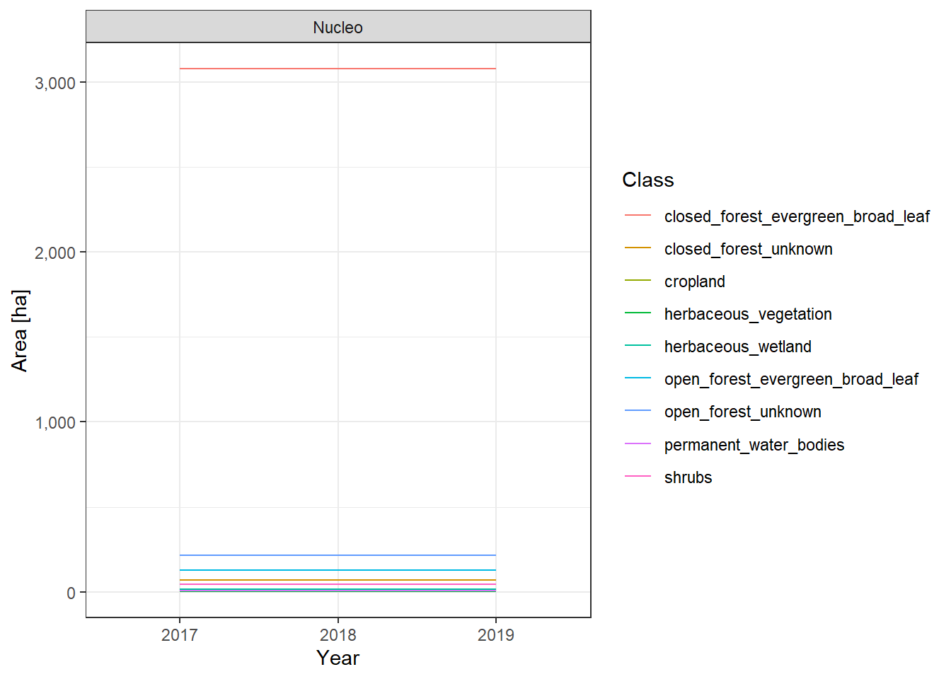
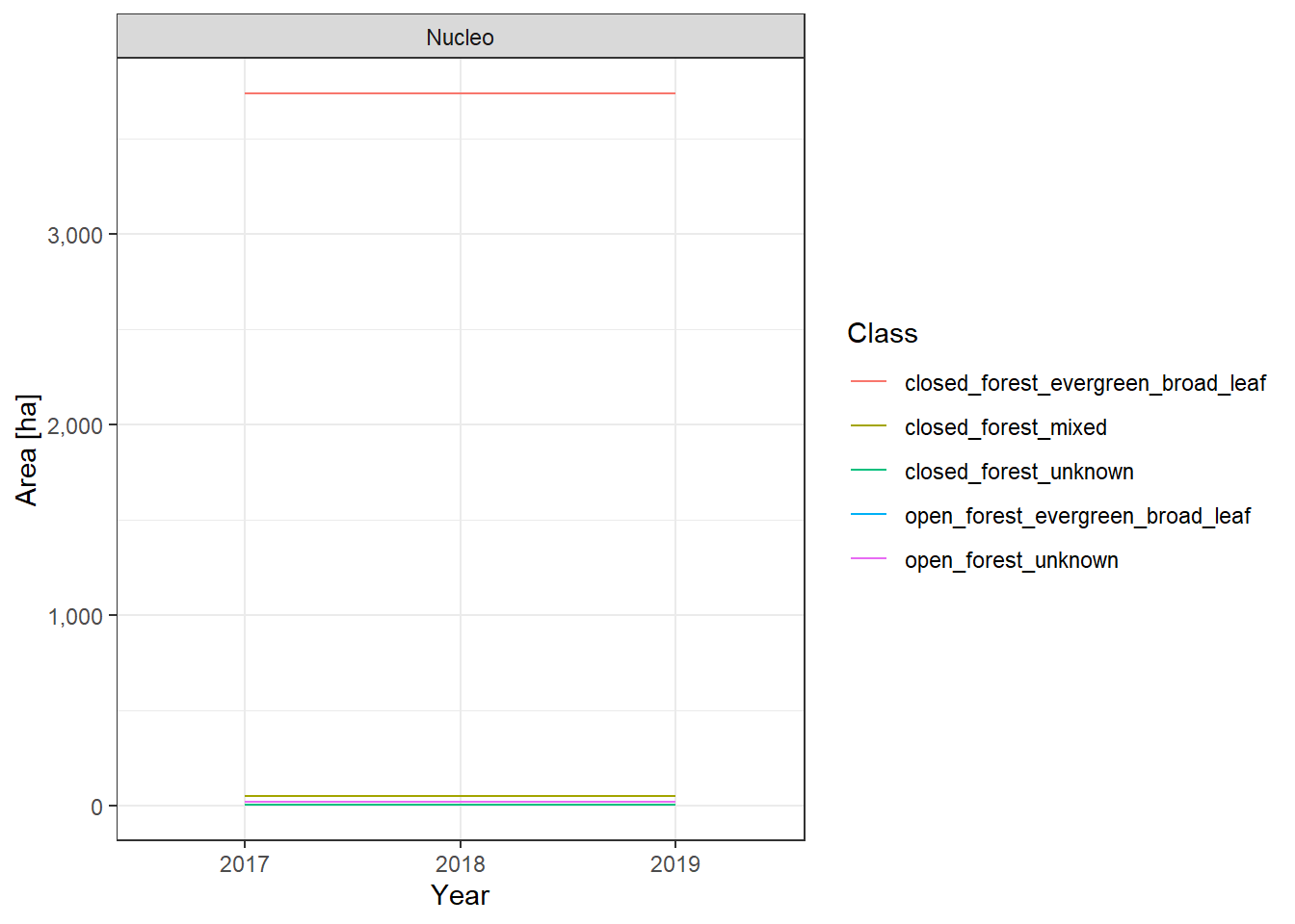
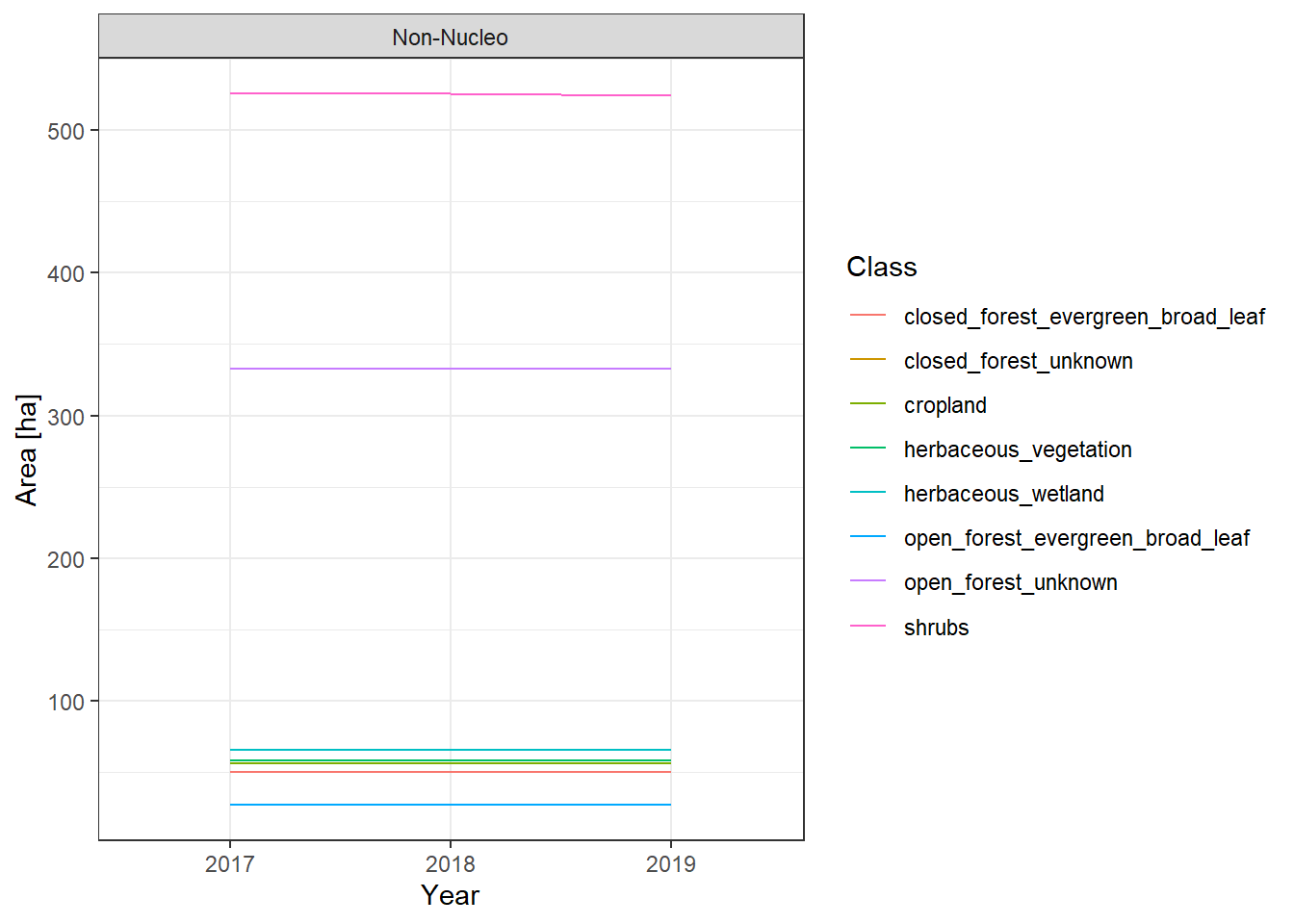
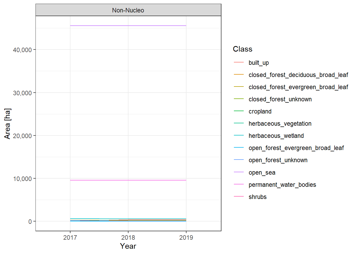
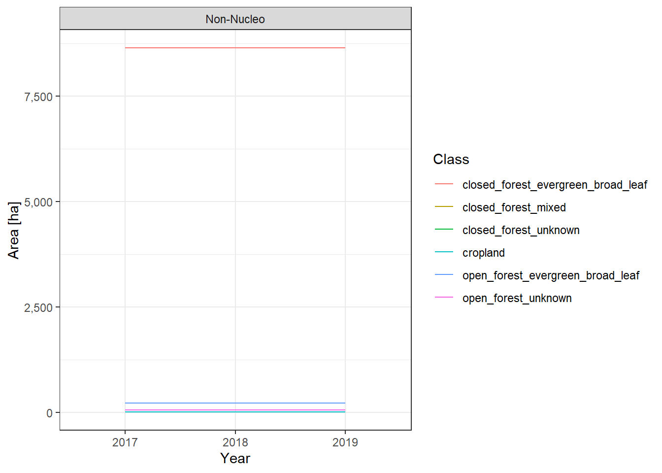
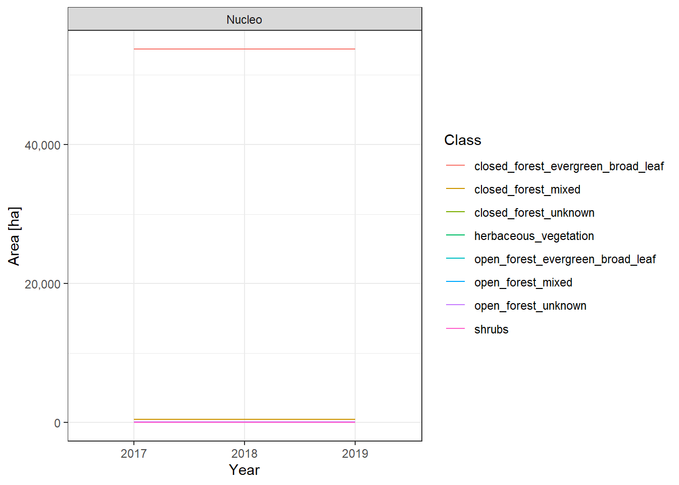
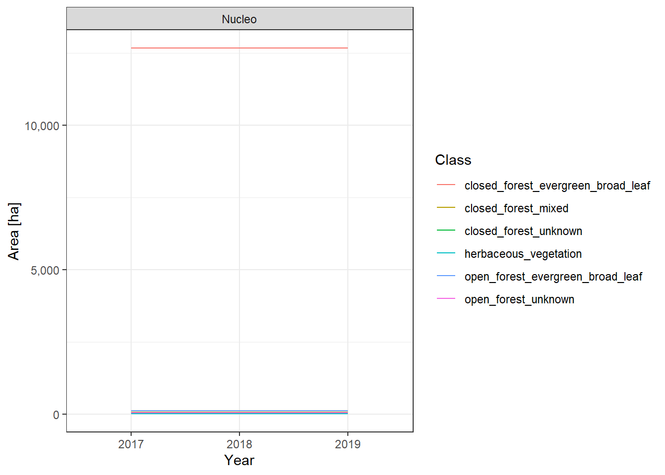
Land Cover changes
The land cover change plots show a lot of different classes on limited space and are therefore hard to distinguish.
To make it easier to interpret the actual numbers, we also include the tabular raw data. The following table lists all land cover classes detected between 2017 and 2019. The Nucleo column indicates, whether a line represents the core zone of a PA or the surrounding area. The column difference_ha shows the absolute area difference of a class between 2017 and 2019. You can interact with the table by clicking on the column titles or typing phrases into the search box. You can also download the data as xlsx or CSV file to use it in a tool of your choice.
Plots
Barras de Cuero y Salado
Capiro y Calentura
Cuyamel
Islas de la Bahia
Omoa
Pico Bonito
Overview Map – Forest and Mangrove Coverage
To explore the changes in forest and mangrove coverage as reported by GFW and GMW, respectively, you can click on a region of your choice, which shows the two time series as a plot.
sessionInfo()R version 4.3.1 (2023-06-16 ucrt)
Platform: x86_64-w64-mingw32/x64 (64-bit)
Running under: Windows 11 x64 (build 22621)
Matrix products: default
locale:
[1] LC_COLLATE=English_United States.utf8
[2] LC_CTYPE=English_United States.utf8
[3] LC_MONETARY=English_United States.utf8
[4] LC_NUMERIC=C
[5] LC_TIME=English_United States.utf8
time zone: Europe/Berlin
tzcode source: internal
attached base packages:
[1] stats graphics grDevices utils datasets methods base
other attached packages:
[1] purrr_1.0.2 sf_1.0-14 scales_1.2.1
[4] reshape2_1.4.4 plotly_4.10.2 ggplot2_3.4.3
[7] mapme.biodiversity_0.4.0 magrittr_2.0.3 leafpop_0.1.0
[10] leaflet.extras2_1.2.2 leaflet.extras_1.0.0 leaflet_2.2.0
[13] htmltools_0.5.6.1 dplyr_1.1.2
loaded via a namespace (and not attached):
[1] tidyselect_1.2.0 viridisLite_0.4.2 farver_2.1.1
[4] fastmap_1.1.1 lazyeval_0.2.2 promises_1.2.1
[7] digest_0.6.33 lifecycle_1.0.3 ellipsis_0.3.2
[10] terra_1.7-39 smoothr_1.0.1 compiler_4.3.1
[13] rlang_1.1.1 sass_0.4.7 tools_4.3.1
[16] utf8_1.2.3 yaml_2.3.7 data.table_1.14.8
[19] knitr_1.44 labeling_0.4.3 brew_1.0-8
[22] htmlwidgets_1.6.2 classInt_0.4-10 curl_5.1.0
[25] plyr_1.8.9 KernSmooth_2.23-22 workflowr_1.7.1
[28] withr_2.5.1 grid_4.3.1 fansi_1.0.4
[31] git2r_0.32.0 e1071_1.7-13 colorspace_2.1-0
[34] future_1.33.0 progressr_0.14.0 globals_0.16.2
[37] cli_3.6.1 rmarkdown_2.25 generics_0.1.3
[40] rstudioapi_0.15.0 httr_1.4.7 DBI_1.1.3
[43] cachem_1.0.8 proxy_0.4-27 stringr_1.5.0
[46] parallel_4.3.1 base64enc_0.1-3 vctrs_0.6.3
[49] jsonlite_1.8.7 listenv_0.9.0 systemfonts_1.0.4
[52] crosstalk_1.2.0 tidyr_1.3.0 jquerylib_0.1.4
[55] units_0.8-4 glue_1.6.2 parallelly_1.36.0
[58] lwgeom_0.2-13 codetools_0.2-19 leaflet.providers_1.13.0
[61] DT_0.30 stringi_1.7.12 gtable_0.3.4
[64] later_1.3.1 munsell_0.5.0 tibble_3.2.1
[67] pillar_1.9.0 furrr_0.3.1 R6_2.5.1
[70] rprojroot_2.0.3 evaluate_0.22 httpuv_1.6.11
[73] bslib_0.5.1 class_7.3-22 Rcpp_1.0.11
[76] uuid_1.1-1 svglite_2.1.1 whisker_0.4.1
[79] xfun_0.40 fs_1.6.3 pkgconfig_2.0.3 UNEP-WCMC and IUCN (2022), Protected Planet: The World Database on Protected Areas (WDPA) and World Database on Other Effective Area-based Conservation Measures (WD-OECM) [Online], February 2022, Cambridge, UK: UNEP-WCMC and IUCN. Available at: www.protectedplanet.net.↩︎
“Bunting, P.; Rosenqvist, A.; Hilarides, L.; Lucas, R.M.; Thomas, T.; Tadono, T.; Worthington, T.A.; Spalding, M.; Murray, N.J.; Rebelo, L-M. Global Mangrove Extent Change 1996 – 2020: Global Mangrove Watch Version 3.0. Remote Sensing. 2022”↩︎
“Hansen, M. C., P. V. Potapov, R. Moore, M. Hancher, S. A. Turubanova, A. Tyukavina, D. Thau, S. V. Stehman, S. J. Goetz, T. R. Loveland, A. Kommareddy, A. Egorov, L. Chini, C. O. Justice, and J. R. G. Townshend. 2013. “High-Resolution Global Maps of 21st-Century Forest Cover Change.” Science 342 (15 November): 850–53. Data available on-line from: http://earthenginepartners.appspot.com/science-2013-global-forest.”↩︎
“ESA. Land Cover CCI Product User Guide Version 2. Tech. Rep. (2017). Available at: maps.elie.ucl.ac.be/CCI/viewer/download/ESACCI-LC-Ph2-PUGv2_2.0.pdf”↩︎